RAG From Scratch – Research to Production
This series bridges the gap between AI research and software engineering. It moves from the high-level intuition of Large Language Models to the low-level systems engineering required to build deterministic, production-grade RAG pipelines.
- Part 1: Revolutionizing Question-and-Answer Systems (RAG Intuition) – The mental model of the “Student” and the “Librarian.”
- Part 2: Building RAG: All Things Retrieval – The basics of Vector Stores and Search.
- Part 3: Deep Dive: Keyword Search – Understanding BM25 and the math of “exact match.”
- Part 4: RAG Systems Engineering: The Structure-Aware Data Pipeline – Fixing the “Garbage In” problem with logical chunking.
- Part 5: Beyond Vectors: Sparse Embeddings & SPLADE – Solving the “Vocabulary Mismatch” problem.
- Part 6: RAG Architecture: The “Union + Rerank” Pipeline – Orchestrating Hybrid Search for production.
In the previous article, we established the basics of chunking, search methods (keyword vs. vector), and Hybrid Search.
Introduction
In information retrieval (IR), a search matches user queries with documents and returns them in a ranked order. This can be analogous to SQL queries for retrieving data, using WHERE clauses to identify rows, and ORDER BY to rank the identified rows. Unlike SQL queries, search engines suggest result ordering based on relevance as users do not specify their preferences.
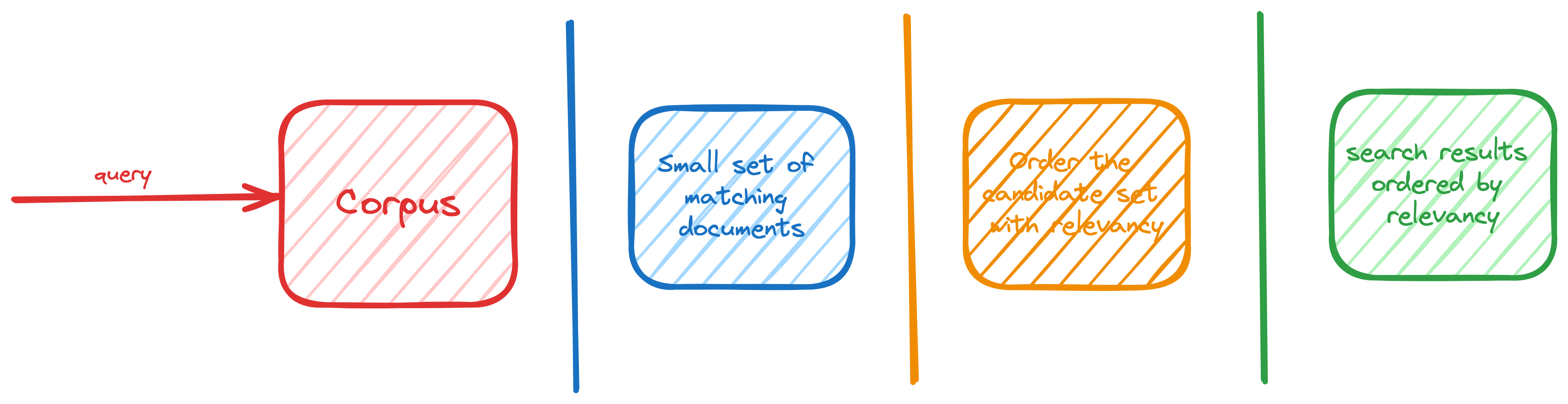
The search retrieval component needs to efficiently identify a small subset of relevant documents based on the user’s query. Once a smaller set of candidate documents is identified, more advanced techniques can be used to order them optimally for the user’s query.
Keyword Search
Conventional keyword search matches user query words to document words using an inverted index data structure for efficient matching and ranking by relevancy.
Inverted Index
To quickly find relevant documents during a search, an inverted index is built in advance. An inverted index is similar to a hashmap, where the keyword serves as the key and the value is a list of matching document references. Using this inverted index, retrieving a list of documents that match one or more keywords present in the search query is faster.
While the inverted index retrieves matching documents for user queries. The ranking function orders the documents based on some scoring function, positioning higher-scored ones at the top of the results list for users.
Ranking functions
Ranking functions like TF-IDF or BM25 reward relevance by assigning scores to documents based on their relevance to the search query. The more relevant a document is the higher its score. We assume that the more a term appears in a document (term frequency (TF)), the more relevant it is. Though this assumption is suboptimal, it proves to be effective enough to be valuable.
TF-IDF
TF-IDF is calculated by multiplying term frequency (TF) with inverse document frequency (IDF). TF measures how often a term appears in a document, while IDF measures how unique a term is across the entire document collection. Multiplying these values gives us the TF-IDF score, indicating a term’s importance within a specific document and the entire collection.
Let’s build some intuition into TF-IDF.
-
Let’s begin developing our ranking function with a straightforward approach. We will assign the score of a document as equal to its term frequency, the number of times the term appears in this document:
score(D, T) = termFrequency(D, T) -
Remember that the queries are free text queries with multiple terms, so the rank can be a sum of all term frequencies. For a given query(Q):
score(D, Q) = sum over all terms T in Q of score(D, T) -
All query terms are treated equally, regardless of their significance. The combined score can be dominated by frequent but insignificant terms like “and” and “the.” This leads to less relevant results appearing first due to the prevalence of filler words.
-
To prevent stop words from dominating, we need to judge the importance of terms in a query. We can’t encode natural language understanding into our scoring function, so we’ll try to find a proxy for importance - rarity. If a term doesn’t occur in most documents, its occurrence is significant. Conversely, if a term occurs in most documents, its presence loses value as an indicator of relevance.
-
Let us update our ranking function in a way that rewards term frequency but penalizes document frequency, we could try dividing TF by DF:
score(D, T) = termFrequency(D, T) / docFrequency(T) -
The issue with DF alone is that it doesn’t provide meaningful information. For instance, if the DF for “dog” is 100, its rarity or commonness depends on the corpus size. In a corpus of 100 documents, the term “dog” is common but if the corpus is 100,000 documents, then it’s rare.
-
Instead of using DF alone, consider \(\frac{N}{DF}\), where N is the index/corpus size. Note how \(\frac{N}{DF}\) is low for common terms (e.g., 100 occurrences of "dog" in a corpus of size 100 would yield \(\frac{N}{DF}\) = 1) and high for rare ones (e.g., 100 occurrences of "dog" in a corpus of size 100,000 would give \(\frac{N}{DF}\) = 1000).
score(D, T) = termFrequency(D, T) * (N / docFrequency(T)) -
Let's examine \(\frac{N}{DF}\). If "dog" appears in 1 out of 100 documents and "cat" in 2, their \(\frac{N}{DF}\) values are 100 and 50 respectively. Should a cat’s score be halved due to its slightly higher frequency?
-
When DF is low, small changes in it greatly affect \(\frac{N}{DF}\) and the score. To smooth out the decline of \(\frac{N}{DF}\) at the lowest end of its range, taking the log of \(\frac{N}{DF}\) can be helpful. Let’s call \(\log\lparen\frac{N}{DF}\rparen\) the inverse document frequency (IDF) of a term.
-
Our ranking function for each term can now be expressed as:
score(D, T) = termFrequency(D, T) * log(N / docFrequency(T))
BM25
BM25 improves upon TF*IDF. BM25 stands for “Best Match 25”. The TF-IDF scoring system does not consider document length and term saturation, which are improved in BM25. Let us continue building BM25 on top of TF-IDF.
-
Term Saturation. TF is important, but too many occurrences of a term shouldn’t significantly impact the score. We want to control TF’s contribution and have a parameter k to shape the saturation curve for experimentation with different values. To achieve this, we’ll pull out a trick. Instead of using raw TF in our ranking formula, we’ll use the value:
termFrequency(D, T) = TF / (TF + k) -
Using \(\frac{TF}{TF + k}\) for term saturation rewards complete matches over partial ones. For example, searching for "cat dog" prefers a document with one instance of each term over a document with two instances of "cat" and none of "dog." This approach ensures that having one instance of each term is always better than having two instances of just one.
-
Document Length. When calculating TF-IDF, consider document length. Reward matches in short documents and penalizes matches in long ones. Use the corpus as a frame of reference for document length. Adjust (TF + k) by multiplying k with the ratio dl/adl, where dl is the document’s length and adl is the average document length across the corpus. This ensures that shorter documents are rewarded while longer documents are penalized, affecting the TF saturation curve accordingly.
termFrequency(D, T) = TF/(TF + k * (dl/adl)) -
The updated term frequency function now considers document length. However, we will introduce a parameter “b” that allows us to experiment with the importance of document length, ranging from 0 to 1. Varying “b” adjusts how the multiplier responds to changes in dl/adl.
termFrequency(D, T) = TF/(TF + k * (1 - b + b * dl/adl)) -
Now it's time to revisit how BM25 handles document frequency. IDF is redefined as \(\log\lparen\dfrac{N-DF+.5}{DF+.5}\rparen\) in BM25, which differs from the previous definition of \(\log\lparen\dfrac{N}{DF}\rparen\). This change stems from efforts to establish a more theoretically grounded ranking function. The Robertson-Spärck Jones weight was simplified to yield \(\log\lparen\frac{N-DF+.5}{DF+.5}\rparen\), known as "probabilistic IDF" when N=10.
-
Probabilistic IDF sharply decreases for terms prevalent in most documents, aiming to reduce the weight of stopwords like “and” or “or.” However, it yields negative values for terms appearing in over half the corpus.
-
To address this, search implementations add 1 to the formula: IDF = \(\log\frac{1 + (N - DF + .5)}{DF + .5}\). Despite seeming minor, this modification effectively reverts the formula to the traditional version: \(\log\lparen\frac{N}{DF}\rparen\).
-
Thus, BM25 ultimately employs the same old version of IDF used in TF-IDF without accelerated decline for high DF values.
score(D, T) = termFrequency(D, T) * log (1 + (N - DF + .5)/(DF + .5))
In summary, TF-IDF simplifies by rewarding term frequency and penalizing document frequency. On the other hand, BM25 transcends this approach by considering document length and term frequency saturation.
Next: RAG Systems Engineering: The Structure-Aware Data Pipeline — we fix the “Garbage In” problem with logical chunking, metadata, and multi-resolution indexing. Read Part 4 here: RAG Systems Engineering