My first GPU-backed run used vLLM’s offline LLM.generate API. The second run put vLLM behind its OpenAI-compatible server and measured streaming TTFT and TPOT. Those experiments showed the runtime from a caller’s point of view. They did not show how serving engines manage memory.
To understand the memory problem, I first needed to follow one request through generation: how the model reads its prompt, produces each new token, and retains useful state from earlier tokens in that same request. Then I could ask how a serving engine handles many requests efficiently.
One Request: Read the Prompt, Then Generate the Answer
Consider the prompt “The cat sat on the”. A tokenizer turns it into token IDs. A token might be a word, part of a word, or punctuation. The full prompt is known when the model starts, so it can process its positions together. This first pass is called prefill.
The model works through a series of layers, or stages of computation, one stage at a time. Within a stage, it can process the prompt’s token positions in parallel because their inputs from the previous stage are already available. Each position is allowed to use only itself and earlier positions; a mask blocks later ones. After processing the prompt, the model predicts a possible next token. In our example, that might be a token representing “ mat” (the exact token boundary depends on the tokenizer).
Now the model needs to predict the token after “ mat”. It could not make that prediction earlier because it did not yet know which token would follow the prompt. It processes the selected token using information retained from the prompt, chooses another token, and repeats. This phase is called decode:
known prompt → prefill → first output token
new token + retained state → decode → next output token (repeat)
The key difference is what the model knows in advance. It has the whole prompt for prefill, but each decode step depends on the token chosen in the previous step. The GPU can do many calculations in parallel within a step, but producing the following token has to wait for that choice. This is the autoregressive generation loop described by the original Transformer paper.
How Attention Finds Earlier Context
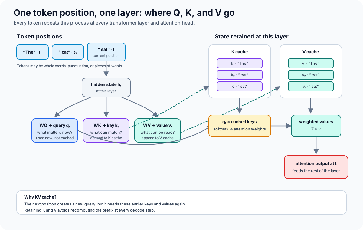
The “earlier context” in that loop is accessed through attention. At each layer, a token position has a hidden-state vector, a numerical representation of that position. Three learned matrices turn it into a query (Q), a key (K), and a value (V):
(q_t, k_t, v_t) = (h_t W_Q, h_t W_K, h_t W_V)
Think of the query as a search vector, each key as something it can match against, and the corresponding value as information to blend into the output. These are learned numerical vectors, not literal words or questions. In the example, the position for “ mat” creates a query that scores the available keys, including those associated with “cat”, “sat”, and its own position. The scores determine how much of each value contributes to the output.
weights = softmax(q_t K_≤tᵀ / sqrt(head_dim))
output = weights V_≤t
Here, t is the position being processed and ≤t means all accessible positions through it. Each layer performs attention across multiple heads. Some architectures share KV heads among query heads, so the number of KV heads need not equal the number of query heads.
Why Cache K and V, but Not Q?
After prefill, the prompt’s keys and values have already been computed. Causal attention prevents later tokens from changing those earlier representations, so their K and V can be reused. Each decode step computes the new position’s Q, K, and V, appends its K and V to the cache, and uses its query to attend over the available history. Future positions have their own queries; old queries are no longer needed. The Hugging Face cache explanation walks through this per-layer reuse.
Caching avoids recomputing the prefix’s representations. Full attention still reads earlier K and V during each step. For one layer, one K or V tensor has a conceptual shape of [sequence_length, num_kv_heads, head_dim]. Both tensors are retained across all layers, so one request’s cache grows as more tokens are processed.
Many Requests: Why the Server Batches GPU Work
Prefill and decode describe the lifetime of one request. Batching is a separate serving decision: combine work from independent requests to make better use of the GPU.
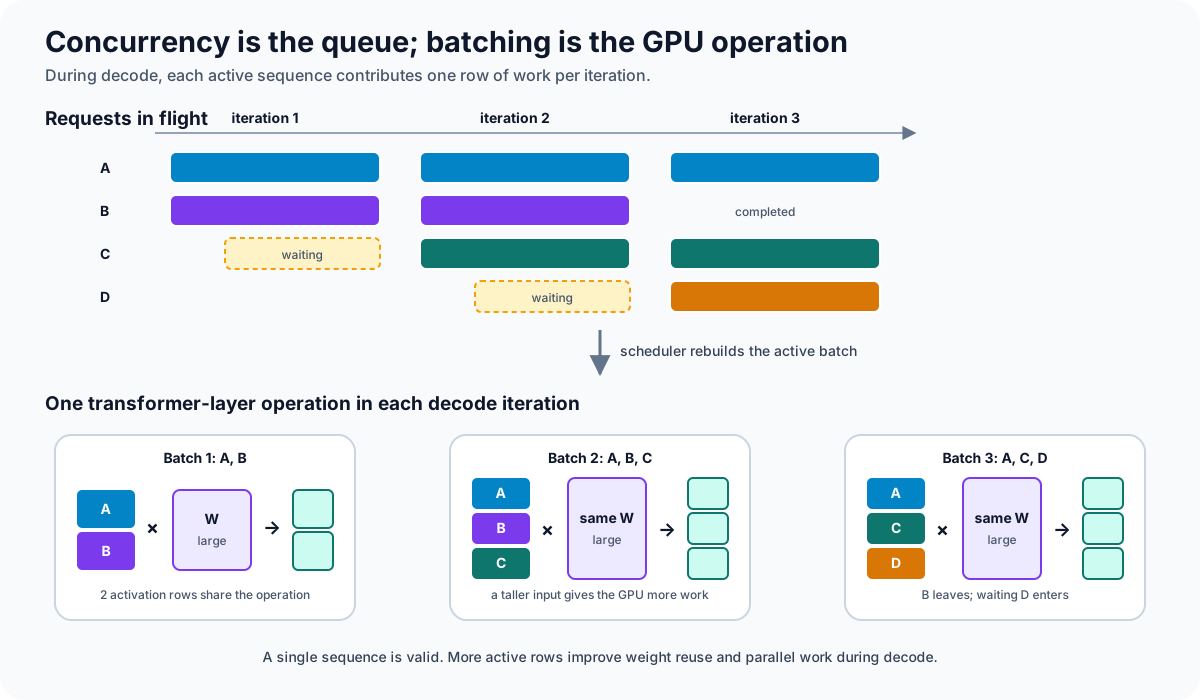
During a decode step, one sequence supplies one activation row to the model’s large weight-matrix operations. At small batch sizes, reading weights from GPU memory can dominate execution while much of the arithmetic capacity goes unused. A batch supplies several rows, allowing weight data to serve more token computations and exposing more parallel work. Each sequence still advances one token at a time; several sequences advance together. NVIDIA’s inference guide explains this compute-versus-memory tradeoff.
Several HTTP requests being in flight does not automatically produce these larger operations. The serving scheduler must select and combine their work. Continuous batching updates the active set between iterations so new requests can join as others finish. Prefill also provides parallel work across prompt positions; the diagram isolates decode to show batching across requests.
The cost consequence follows from how we pay for capacity. For rented GPUs, a useful accounting measure is:
GPU cost per useful output token =
    GPU rental cost over an interval / useful output tokens delivered in that interval
If a busy service leaves hardware capacity unused, it delivers fewer tokens for that spend and may need more GPUs for the same demand. Batching can improve throughput, but larger batches can also increase latency. The target is useful output within the service’s latency limits, rather than the largest possible batch.
Every active sequence also needs its KV cache. That connects GPU efficiency to allocation: wasted cache capacity can limit the requests available to batch, even with a full queue. The next experiment isolates that memory constraint; it does not measure a throughput or cost improvement.
The PagedAttention paper by Kwon et al., published at SOSP 2023, reports that prior serving systems may use only 20% to 38% of reserved KV-cache memory for actual token state. I built a small allocation simulation to make one part of that claim concrete: the difference between reserving a worst-case buffer for every request and allocating capacity in fixed-size blocks.
The Reservation Baseline
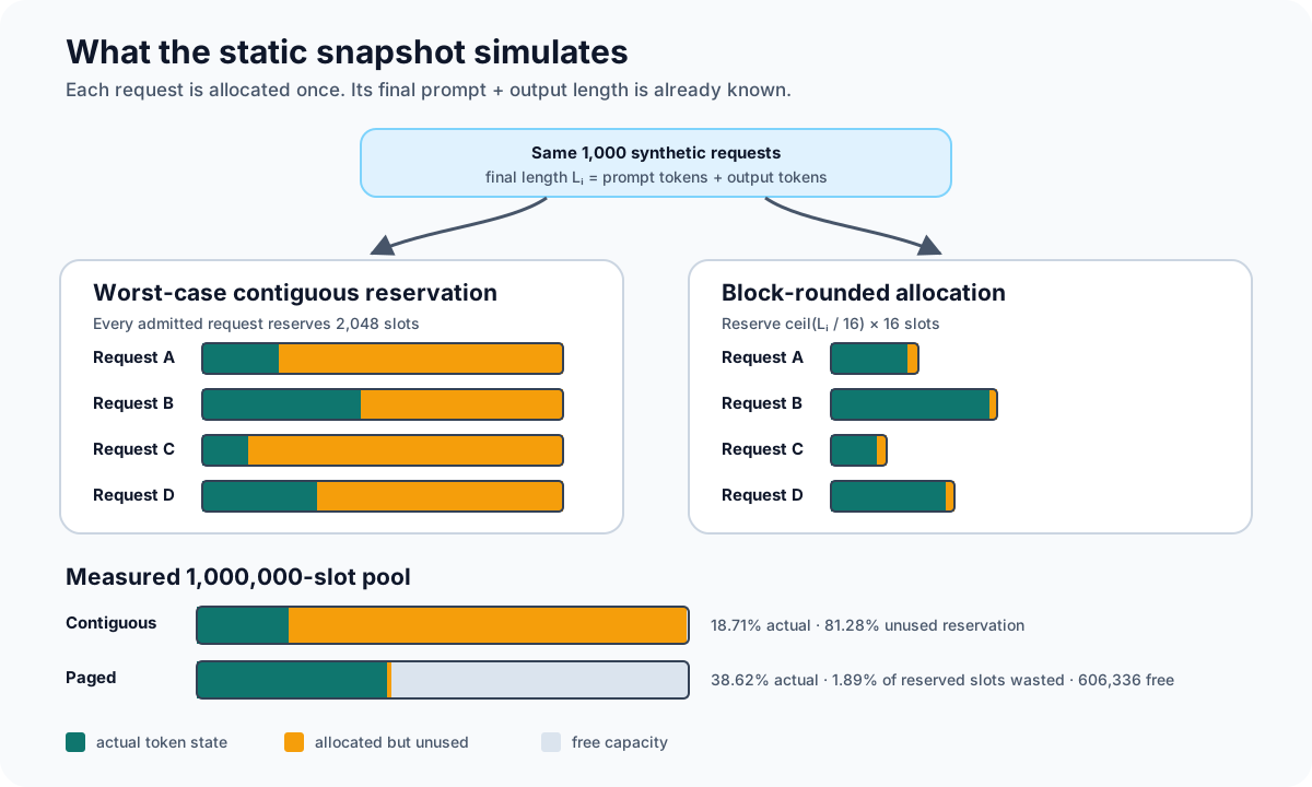
The simulator abstracts the per-layer K and V tensors described above into token slots. A simple baseline reserves max_seq_len such slots for every admitted request.
Worst-case reservation is easy to reason about, but it wastes capacity when final sequence lengths are much shorter than the limit. A request that ultimately contains 200 tokens still occupies a 2048-slot reservation.
Other memory-management problems require a request lifecycle to observe. External fragmentation requires allocations and frees that leave holes which cannot serve later allocation sizes. Prefix sharing and copy-on-write require multiple related sequences. This first simulation includes neither behavior.
What Paged Allocation Changes
In the paper’s system, physical KV-cache memory is divided into fixed-size blocks. Each sequence has a block table that maps logical blocks to physical blocks, so logically adjacent tokens do not require physically adjacent storage. The PagedAttention kernel follows that mapping while computing attention.
The block table supplies indirection. The serving runtime around the kernel manages the free-block pool, admission, reference counts, copy-on-write, preemption, and any swapping policy. Keeping those responsibilities separate matters: PagedAttention is the attention algorithm that can consume non-contiguous KV blocks; it is not, by itself, the entire allocator and scheduler.
The Static Snapshot
The pure-Python harness compares two strategies on the same synthetic workload:
- Contiguous reservation: reserve
max_seq_lenslots for each request. - Paged allocation: round each request’s final length up to a whole number of fixed-size blocks.
The workload contains 1000 requests. Prompt lengths are sampled uniformly from 50 to 500 tokens and output lengths from 20 to 200 tokens. The configured KV budget is 1,000,000 abstract token slots.
Every request is allocated once using its already-known final prompt-plus-output length. The harness does not grow requests during decoding, free completed requests, model arrival times or preemption, share prefixes, perform copy-on-write, evict blocks, or swap them. This is a static allocation snapshot rather than a serving trace.
The synthetic input is deterministic. This is the complete request definition and workload generator behind the reported run:
import random
from dataclasses import dataclass

@dataclass(frozen=True)
class Request:
    req_id: int
    prompt_tokens: int
    output_tokens: int

    @property
    def total_tokens(self):
        return self.prompt_tokens + self.output_tokens

rng = random.Random(42)
requests = [
    Request(i, rng.randint(50, 500), rng.randint(20, 200))
    for i in range(1000)
]
The contiguous strategy searches for max_seq_len adjacent free slots and reserves the entire run. It rejects a request whose known final length exceeds that reservation limit:
def allocate(self, req):
    if req.total_tokens > self.max_seq_len:
        raise ValueError("request exceeds max_seq_len")
    start = self.find_contiguous_free_run(self.max_seq_len)
    if start is None:
        return False
    for slot in range(start, start + self.max_seq_len):
        self.memory[slot] = req.req_id
    self.allocations[req.req_id] = (start, start + self.max_seq_len)
    return True
The paged strategy rounds the same final length to blocks and can draw those blocks from anywhere in its free pool:
class PagedAllocator:
    def __init__(self, total_tokens: int, block_size: int):
        self.block_size = block_size
        self.num_blocks = total_tokens // block_size
        self.free_blocks = list(range(self.num_blocks))
        self.allocations = {}

    def allocate(self, req):
        needed = (req.total_tokens + self.block_size - 1) // self.block_size
        if len(self.free_blocks) < needed:
            return False
        blocks = [self.free_blocks.pop() for _ in range(needed)]
        self.allocations[req.req_id] = blocks
        return True
For example, a 20-token request needs two 16-token blocks. Executing this excerpt leaves the allocator with two block IDs assigned to that request.
The Numbers
| Metric | Contiguous | Paged (block size 16) |
|---|---|---|
| Admitted requests | 488 | 1000 |
| Actual token slots | 187,131 | 386,241 |
| Reserved token slots | 999,424 | 393,664 |
| Free token slots | 576 | 606,336 |
| Utilization | 18.71% | 38.62% |
| Internal fragmentation | 81.28% | 1.89% |
| History-induced external fragmentation | 0.00% | 0.00% |
The denominators differ. Utilization is actual token slots divided by the allocator’s usable pool. It describes token-slot occupancy, not GPU compute utilization or serving throughput. Internal fragmentation is unused allocated slots divided by reserved slots. It is therefore not the complement of utilization; free capacity is a separate quantity.
The contiguous strategy admits 488 requests and reserves 999,424 slots for 187,131 actual tokens. Paged allocation admits all 1000 requests and reserves 393,664 slots for 386,241 actual tokens. On this workload, block rounding limits unused space to the tail of each request’s final block.
Zero external fragmentation is expected here. The snapshot never frees a request, and every contiguous reservation has the same 2048-slot size. Finishing one such request would release a complete 2048-slot reservation that another equal-size reservation could reuse. These results do not demonstrate recovery from fragmented memory.
What the Block-Size Sweep Measures
| Block size | Internal fragmentation |
|---|---|
| 8 | 0.89% |
| 16 | 1.89% |
| 32 | 3.87% |
| 64 | 7.55% |
| 128 | 14.28% |
This sweep measures only the fragmentation side of the block-size tradeoff. Eight-token blocks have the least tail waste among the tested sizes. The simulation does not measure metadata bytes, lookup overhead, kernel latency, or throughput, so it cannot identify an overall optimum.
The paper uses 16-token blocks as its default and evaluates block size together with GPU execution efficiency in Section 7.2. That historical design choice is broader than what this simulation measures and should not be read as a universal setting for current runtimes.
At block size 128, the allocator can use 999,936 of the configured 1,000,000 slots because it rounds the pool down to whole blocks. The utilization shown as 38.63% rather than 38.62% comes from that smaller denominator; the allocator did not store additional tokens.
A Lifecycle Follow-Up
I followed the snapshot with one deterministic 64-slot lifecycle trace. It contains seven arrivals, four decode-growth events, and two completions. The contiguous baseline reserves 16 slots per admitted request; the paged strategy adds 4-slot blocks as each sequence grows.
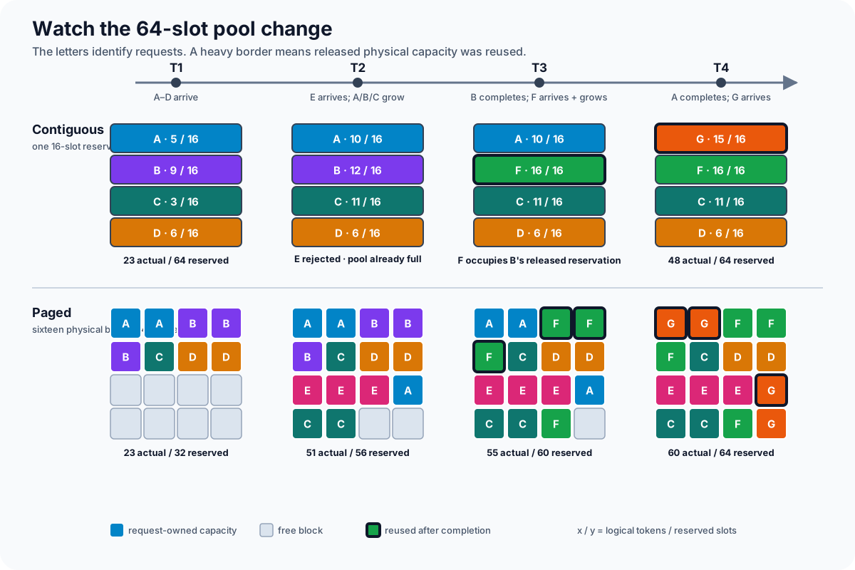
Read each column as the same instant in the two allocators. The upper row shows four physical 16-slot reservations; 10 / 16, for example, means ten logical tokens occupy a sixteen-slot reservation. The lower row shows the actual sixteen-block physical pool. New blocks appear only when growth crosses a four-token boundary. Heavy outlines show F taking B’s released blocks and G taking A’s released blocks.
The main transition happens at T2. The contiguous pool has already committed all 64 slots to A–D, so it rejects E even though those requests contain only 23 logical tokens when E arrives. The paged pool has reserved only 32 slots at that point, so E fits. T3 and T4 then show why external fragmentation remains zero in this experiment: every released reservation or block is reusable.
These are the exact events applied to both allocators:
trace = [
    ("arrive", "A", 5),  ("arrive", "B", 9),
    ("arrive", "C", 3),  ("arrive", "D", 6),
    ("arrive", "E", 12), ("grow", "A", 5),
    ("grow", "B", 3),    ("grow", "C", 8),
    ("complete", "B", 0), ("arrive", "F", 12),
    ("grow", "F", 4),    ("complete", "A", 0),
    ("arrive", "G", 15),
]
| Metric | Contiguous reservations | Paged blocks |
|---|---|---|
| Arrivals admitted | 6 of 7 | 7 of 7 |
| Final active tokens | 48 | 60 |
| Final reserved slots | 64 | 64 |
| Final internal fragmentation | 25.00% | 6.25% |
| Released slots later reused | 32 | 24 |
| History-induced external fragmentation | 0 | 0 |
The contiguous pool filled after four arrivals and rejected the fifth. Once two earlier requests completed, two later arrivals reused both released reservations. Paged allocation admitted the fifth request using capacity that worst-case reservation had already committed, added blocks only when growth crossed a four-token boundary, and reused released blocks after completions.
The zero external-fragmentation result is the point of retaining equal-sized reservations: allocation history did not make either released 16-slot unit unusable. A variable-sized reservation experiment would answer a different question.
The Systems Bridge
The virtual-memory analogy is useful when each responsibility stays concrete:
| Component | Responsibility |
|---|---|
| Block table | Map a sequence’s logical token blocks to physical KV blocks. |
| PagedAttention kernel | Read K and V through that mapping while computing attention. |
| Runtime memory manager | Allocate and reclaim blocks; manage reference counts and copy-on-write where supported. |
| Scheduler | Admit, preempt, and resume requests according to available capacity and policy. |
Fixed-size physical blocks remove the need for each sequence’s KV state to occupy one contiguous physical region. Sharing is possible when the runtime lets multiple logical block tables reference the same physical blocks. The table enables that reference pattern; the runtime must implement its ownership rules.
Where This Analogy Breaks
A general-purpose allocator handles byte-level requests of many sizes. This simulation counts token slots whose per-token KV shape is fixed for one model configuration. Translating those slots into GPU bytes requires the number of layers, both K and V tensors, KV heads, head dimension, and data type.
An operating-system pager can move pages to slower storage with a very different latency budget. The system in the PagedAttention paper includes CPU swapping as a runtime policy under pressure. Swapping is not an intrinsic behavior of every kernel or every runtime that uses paged KV layouts.
The simulation also says nothing about the cost of indirection. In the paper’s historical microbenchmark, the PagedAttention kernel had 20% to 26% higher latency than a highly optimized contiguous attention baseline, while end-to-end serving benefited from better memory use and batching opportunities (PagedAttention Section 7.2). Those are paper results, not measurements from this Python harness.
What I Know Now
The supported result is narrow and useful: when every request reserves its worst-case sequence length, reservation waste dominates this synthetic workload. Rounding known final lengths to blocks reduces that waste and bounds each request’s unused tail.
The lifecycle simulation now makes allocation, growth, completion, and reuse visible, but it does not establish how a live runtime implements them. The next experiment is a pinned vLLM trace that connects those events to the real memory manager and scheduler. Prefix sharing, copy-on-write, and eviction remain beyond these simulations.
Paged allocation answers how KV can be laid out within a worker. It does not decide where prefill and decode execute. That is the disaggregated-serving question, and the two mechanisms can be combined.
Reproducing the Arithmetic
The inputs, seed, allocation rules, lifecycle events, and measured outputs are embedded above so the evidence does not depend on access to a separate repository. The two reported percentages use these formulas:
utilization_pct = actual_tokens / usable_pool_tokens * 100
internal_frag_pct = (reserved_tokens - actual_tokens) / reserved_tokens * 100
For the static paged run, reserved_tokens is the sum of ceil(request.total_tokens / block_size) * block_size over admitted requests. For the contiguous run, it is admitted_requests * max_seq_len. Free capacity remains separate from both percentages.